|
1
|
|
|
2
|
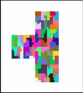
- What is load-balancing?
- Dividing up the total work between processes when running codes on a
parallel machine
- Load-balancing constraints
- Minimize interprocess communication
- Also called:
- partitioning, mesh partitioning, (domain decomposition)
|
|
3
|
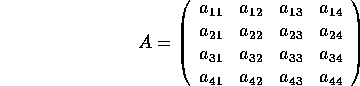
- Memory is organized by banks. Between access to any bank, there is a
latency period.
- Matrix entries are stored
column-wise in FORTRAN.
|
|
4
|
|
|
5
|
- For illustration purposes, lets imagine 8 banks [128 or 256 common on
chips today], with bank busy time (bbt) of 8 cycles between accesses.
Thus we have:
- data a13 a23 a33
a43 a14 a24
a34 a44
- data a11 a21 a31
a41 a12 a22
a32 a42
- bank 1 2 3 4 5 6 7 8
|
|
6
|
- If we access data column-wise, we proceed through each bank in order. By
the time we call a13, we (just) avoid bbt.
- On the other hand, if we access data row-wise, we get a11 in bank 1, a12
in bank 5, a13 in bank 1 again - so instead of access on clock cycle 3,
we have to wait until cycle 9. Then we get a14 in bank 5 again on cycle
10, etc.
|
|
7
|
- If addressing is indirect we may wind up jumping all over, and suffer
performance hits because of it.
|
|
8
|
- Bank conflicts depend on granularity of memory
- If N memory refs per cycle, p processors, memory with b cycles bbt, need
p*N*b memory banks to see uninterrupted access of data
- With B banks, granularity is
- g = B/(p*N*b)
|
|
9
|
- Separate selection of data from its processing
- Each subtask requires its own data structure. Be prepared to change
structures between tasks
|
|
10
|
|
|
11
|
|
|
12
|
- Need a good measure of what the expected work may be
- Molecular dynamics:
- number of molecules
- regions
- FEM/finite difference/finite volume, etc:
- Degrees of freedom
- Cells/elements
- If edge weights are used, also need a good measure on how strongly
objects are coupled to each other
|
|
13
|
- Static load-balancing
- Done as a “preprocessing” step before the actual calculation
- If the objects and edges don’t change very much or at all, can do
static load-balancing
- Dynamic load-balancing
- Done during the calculation
- Significant changes in the objects and/or edges
|
|
14
|
|
|
15
|
- Static partitioning insufficient for many applications
- Adaptive mesh refinement
- Multi-phase/Multi-physics computations
- Particle simulations
- Crash simulations
- Parallel mesh generation
- Heterogeneous
computers
- Need dynamic load balancing
|
|
16
|
- Minimize load-balancing time
- Minimize data migration -- incremental partitions
- Small changes in the computation should result in small changes in the
partitioning
- Calculating new partition and data migration should take less time than
the amount of time saved by performing computations on new grid
- Done in parallel
|
|
17
|
- Geometric
- Based on geometric location
- Faster load-balancing time with medium quality results
- Graph-based
- Create a graph to represent the objects and their connections
- Slower load-balancing time but high quality results
- Incremental methods
- Use graph representation and “shuffle” around objects
|
|
18
|
- No algorithm/method is appropriate for all applications!
- Graph load-balancing algorithms for:
- Static load-balancing
- Computations where computation to load-balancing time ratio is high
- Implicit schemes with a linear and non-linear solution scheme
|
|
19
|
- Geometric load-balancing algorithms for:
- Computations where computation to load-balancing time ratio is low
- For explicit time stepping calculations with many time steps and
varying workload (MD, FEM crash simulations, etc.)
- Problems with many load-balancing objects
|
|
20
|
- Based on the objects’ coordinates
- Want a unique coordinate associated with an object
- Node coordinates, element centroid, molecule coordinate/centroid, etc.
- Partition “space” which results in a partition of the load-balancing
objects
- Edge cuts are usually not explicitly dealt with
|
|
21
|
- Objects that are close will likely need to share information
- Want compact partitions
- High volume to surface area or high area to perimeter length ratios
- Coordinate information
- Bounded domain
|
|
22
|
- Recursive Coordinate Bisection (RCB)
- Recursive Inertial Bisection (RIB)
- Space Filling Curves (SFC)
- Warren & Salmon, Ou, Ranka, & Fox, Baden & Pilkington
- Octree Partitioning/Refinement-tree Partitioning
|
|
23
|
- Choose an axis for the cut
- Find the proper location of the cut
- Group objects together according to location relative to cut
- If more partitions are needed, go to step 1
|
|
24
|
- Choose a direction for the cut
- Find the proper location of the cut
- Group objects together according to location relative to cut
- If more partitions are needed, go to step 1
|
|
25
|
|
|
26
|
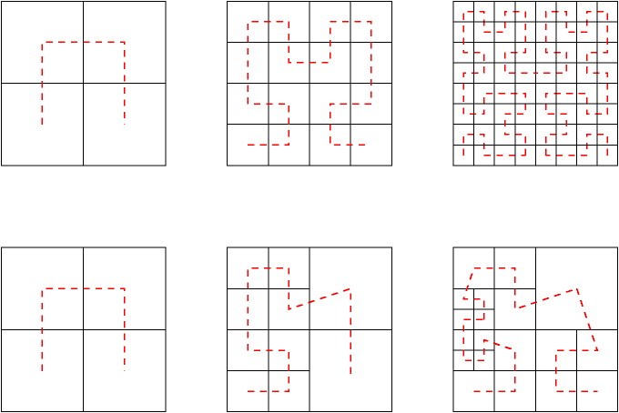
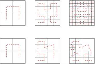
- The SFC gives a 1-dimensional ordering of objects located in an
n-dimensional domain
- Easier to work with objects in 1 dimension than in n dimensions
- Algorithm:
- Sort objects by their location on the SFC
- Calculate cuts along the SFC
|
|
27
|
- Tree based algorithms for applications with multiple levels of data,
simulation accuracy, etc.
- Tree is usually built from specific computational schemes
- Tightly coupled with the simulation
|
|
28
|
- RCB and RIB usually give slightly better partitions than SFC
- SFC is usually a little faster
- SFC is a little better for incremental partitions
- RIB can be real unstable for incremental partitions
|
|
29
|
- There are many load-balancing libraries downloadable from the web
- Mostly graph partitioning libraries
- Static: Chaco, Metis, Party,
Scotch
- Dynamic: ParMetis, DRAMA,
Jostle, Zoltan
- Zoltan (www.cs.sandia.gov/Zoltan)
- Dynamic load-balancing library with:
- SFC, RCB, RIB, Octree, ParMetis, Jostle
- Same interface to all load-balancing algorithms
|
|
30
|
- Avoiding load-balancing
- Load-balancing not needed every time the workload and/or edge
connectivity changes
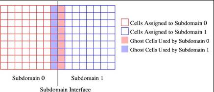
- Ghost cells
- Predictive load-balancing
|
|
31
|
- Need communication between processors
- Use ‘ghost’ cells – need to maintain consistency of data in ghost cells
|
|
32
|
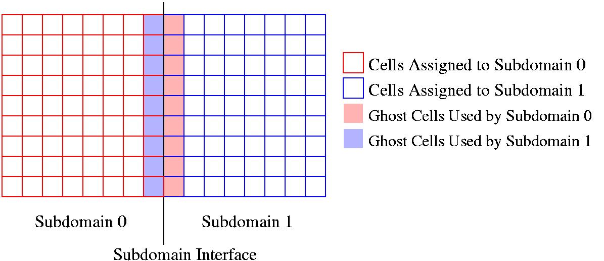
- Copies of cells assigned to other processors
- Make needed information available
- No solution values are computed at the ghost cells
- Ghost cell information needs to be updated whenever necessary
- Ghost cells need to be calculated dynamically because of changing mesh
and dynamic load-balancing
|
|
33
|
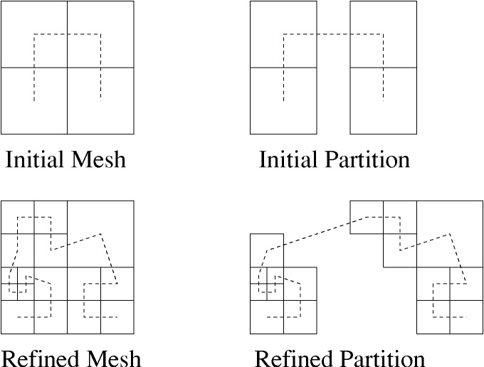
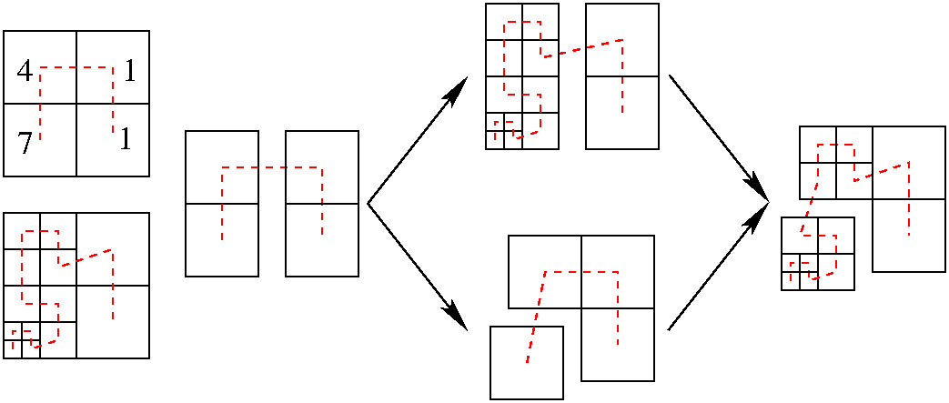
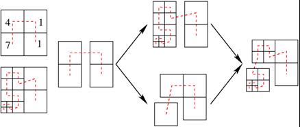
- Predict the workload and/or edge connectivity and load-balance with that
information
- Assumes that you can predict the workload and/or edge connectivity
- Still need to perform communication but reduces data migration
|
|
34
|
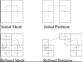
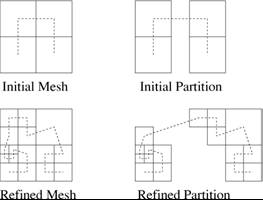
- Refine then load-balance – 4 objects migrated
- Predictive load-balance then refine – 1 object migrated
|

 Notes
Notes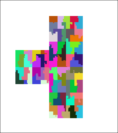