1	Parallelization Strategies and Load Balancing Some material borrowed from lectures of J. Demmel, UC Berkeley
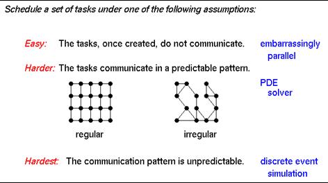
2	Ideas for dividing work Embarrassingly parallel computations ‘ideal case’. after perhaps some initial communication, all processes operate independently until the end of the job examples: computing pi; general Monte Carlo calculations; simple geometric transformation of an image static or dynamic (worker pool) task assignment
3	Ideas for dividing work Partitioning partition the data, or the domain, or the task list, perhaps master/slave examples: dot product of vectors; integration on a fixed interval; N-body problem using domain decomposition static or dynamic task assignment; need for care
4	Ideas for dividing work Divide & Conquer recursively partition the data, or the domain, or the task list examples: tree algorithm for N-body problem; multipole; multigrid usually dynamic work assignments
5	Ideas for dividing work Pipelining a sequence of tasks performed by one of a host of processors; functional decomposition examples: upper triangular linear solves; pipeline sorts usually dynamic work assignments
6	Ideas for dividing work Synchronous Computing same computation on different sets of data; often domain decomposition examples: iterative linear system solves often can schedule static work assignments, if data structures don’t change
7	Load balancing Determined by Task costs Task dependencies Locality needs Spectrum of solutions Static - all information available before starting Semi-Static - some info before starting Dynamic - little or no info before starting Survey of solutions How each one works Theoretical bounds, if any When to use it
8	Load Balancing in General Large literature A closely related problem is scheduling, which is to determine the order in which tasks run
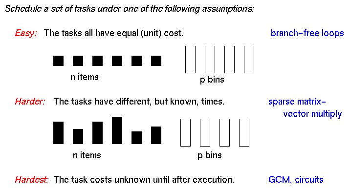
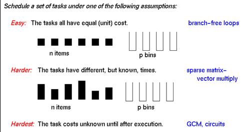
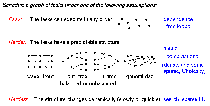
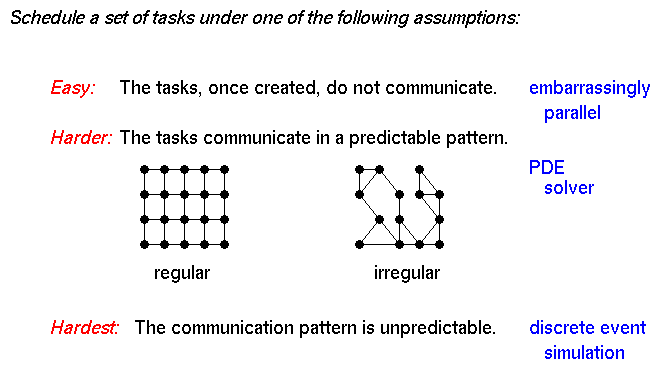
9	Load Balancing Problems Tasks costs Do all tasks have equal costs? Task dependencies Can all tasks be run in any order (including parallel)? Task locality Is it important for some tasks to be scheduled on the same processor (or nearby) to reduce communication cost?
10	Task cost spectrum
11	Task Dependency Spectrum
12	Task Locality Spectrum
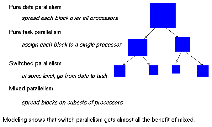
13	Approaches Static load balancing Semi-static load balancing Self-scheduling Distributed task queues Diffusion-based load balancing DAG scheduling Mixed Parallelism
14	Static Load Balancing All information is available in advance Common cases: dense matrix algorithms, e.g. LU factorization done using blocked/cyclic layout blocked for locality, cyclic for load balancing usually a regular mesh, e.g., FFT done using cyclic+transpose+blocked layout for 1D sparse-matrix-vector multiplication use graph partitioning, where graph does not change over time
15	Semi-Static Load Balance Domain changes slowly; locality is important use static algorithm do some computation, allowing some load imbalance on later steps recompute a new load balance using static algorithm Particle simulations, particle-in-cell (PIC) methods tree-structured computations (Barnes Hut, etc.) grid computations with dynamically changing grid, which changes slowly
16	Self-Scheduling Self scheduling: Centralized pool of tasks that are available to run When a processor completes its current task, look at the pool If the computation of one task generates more, add them to the pool Originally used for: Scheduling loops by compiler (really the runtime-system)
17	When is Self-Scheduling a Good Idea? A set of tasks without dependencies can also be used with dependencies, but most analysis has only been done for task sets without dependencies Cost of each task is unknown Locality is not important Using a shared memory multiprocessor, so a centralized pool of tasks is fine
18	Variations on Self-Scheduling Don’t grab small unit of parallel work. Chunk of tasks of size K. If K large, access overhead for task queue is small If K small, likely to have load balance Four variations: Use a fixed chunk size Guided self-scheduling Tapering Weighted Factoring
19	Variation 1: Fixed Chunk Size How to compute optimal chunk size Requires a lot of information about the problem characteristics e.g. task costs, number Need off-line algorithm; not useful in practice. All tasks must be known in advance
20	Variation 2: Guided Self-Scheduling Use larger chunks at the beginning to avoid excessive overhead and smaller chunks near the end to even out the finish times.
21	Variation 3: Tapering Chunk size, K_i is a function of not only the remaining work, but also the task cost variance variance is estimated using history information high variance => small chunk size should be used low variant => larger chunks OK
22	Variation 4: Weighted Factoring Similar to self-scheduling, but divide task cost by computational power of requesting node Useful for heterogeneous systems Also useful for shared resource e.g. NOWs as with Tapering, historical information is used to predict future speed “speed” may depend on the other loads currently on a given processor
23	Distributed Task Queues The obvious extension of self-scheduling to distributed memory Good when locality is not very important Distributed memory multiprocessors Shared memory with significant synchronization overhead Tasks that are known in advance The costs of tasks is not known in advance
24	DAG Scheduling Directed acyclic graph (DAG) of tasks nodes represent computation (weighted) edges represent orderings and usually communication (may also be weighted) usually not common to have DAG in advance
25	DAG Scheduling Two application domains where DAGs are known Digital Signal Processing computations Sparse direct solvers (mainly Cholesky, since it doesn’t require pivoting). Basic strategy: partition DAG to minimize communication and keep all processors busy NP complete, so need approximations Different than graph partitioning, which was for tasks with communication but no dependencies
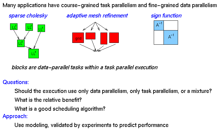
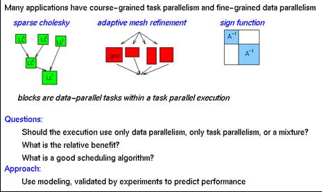
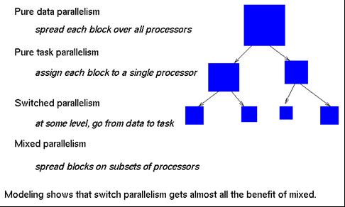
26	Mixed Parallelism Another variation - a problem with 2 levels of parallelism course-grained task parallelism good when many tasks, bad if few fine-grained data parallelism good when much parallelism within a task, bad if little
27	Mixed Parallelism Adaptive mesh refinement Discrete event simulation, e.g., circuit simulation Database query processing Sparse matrix direct solvers
28	Mixed Parallelism Strategies
29	Which Strategy to Use
30	Switch Parallelism: A Special Case
31	A Simple Performance Model for Data Parallelism
32	Values of Sigma - problem size